
-

Sequels: Hubris, Distraction, and Obsession
What makes a game franchise live or die? Most discussion about game franchise deaths are by players and press. Sometimes, there are industry post mortems. Rarely, developers complain about management or team. My career intersects four 20+ year game franchises: Tribes, Marble Blast, Zap, and Blockland. Over the decades, I’ve had time to reflect on those franchises: what worked, and what didn’t.…
-
AI Narratives: Shooting the Script (Part 3)
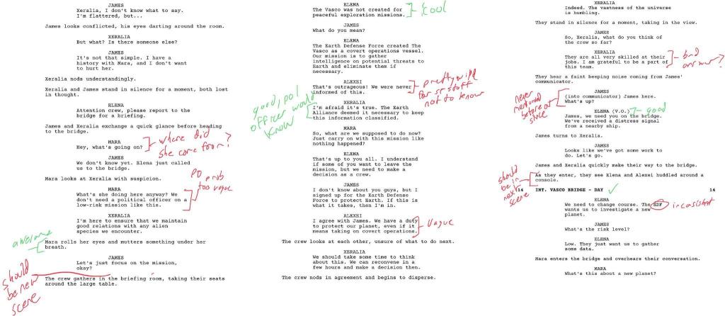
(This is part 3 of a series on an AI generated TV show. Click here to check out part 2.) We’ve covered a lot of ground – from high level concept to a finished script. But a script isn’t very compelling – we need to film it! The video production process mimics Hollywood productions, because it operates under similar constraints: The AI…
-
AI Narratives: Orchestrating a Story (Part 2)
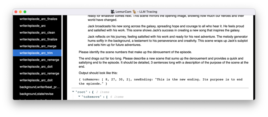
(This is part 2 of a series on an AI generated TV show. Click here to check out part 1.) (Also – Part 3 is available!) So, what do I mean when I say “the AI writes the story”? My narrative generation strategy follows these steps: Let’s dive in! Building Foundations I wrote a library for managing LLM requests, and a tool…
-
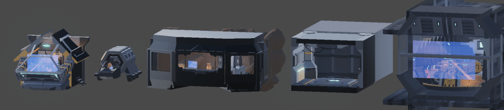
AI Narratives: On Screen! (Part 1)
(This is part 1 of a series. Part 2 is available now!) I made an autonomous space opera generator called On Screen!. Give it a topic, and it generates a 10-15 minute episode ready for upload to YouTube. Let me tell you about it and the journey behind it. January 2023: LLMs start to deliver on natural language AI. Influencers predict the…
-

Marbling It Up
@MarbleItUp has gone public. We will be launching soon on Switch. I wanted to talk a little bit about the game and how it came to be… and share some sweet GIFs (in high framerate black and white for download size reasons). Just over a year ago, Mark Frohnmayer came to me with a proposal – let’s build a sweet marble game and…
-
Video Conference Part 4: Making RANS the Ryg way
Last post, we got our networking stack up and running, figured out how to work around firewalls, and saw how our codec performs over a real network link. This motivated us to revisit our compression schemes, which is what we’ll do in today’s post. We’ll start with some algorithmic improvements to reduce the amount of data we need, then implement an entropy…
-

Video Conference Part 3: Getting Online
Last time we got up close and intimate with the core compression techniques used in the JPEG format, and applied them to our own situation for better compression. We got our data rates low enough that we have a shot at realtime video under ideal network conditions. Now it’s time to actually send data over a network (or at least loopback)! The…
-
Video Conference Part 2: Joint Photographic Hell (For Beginners)
Last time, I got angry at Skype and metaphorically flipped the table by starting to write my own video conference application. We got a skeleton of a chat app and a video codec up, only to find it had a ludicrous 221 megabit bandwidth requirement. We added some simple compression but didn’t get much return from our efforts. We definitely need better compression before…
-

Video Conference Part 1: These Things Suck
What I cannot create, I do not understand. – Richard Feynman I do a lot of video chat for work. If it’s not a one on one, it’s pair programming. If it’s not pair programming, it’s a client meeting. I use a lot of Skype and Hangouts. Sometimes they don’t work for unclear reasons. Sometimes file transfers fail. Sometimes screenshare breaks, or…
-
Huffman Serialization Techniques
Networking expert Glenn Fielder’s article on network serialization techniques is a great read. It discusses a number of scenarios including serializing a sparse set of items from an array. This blog post discusses Glenn’s implementation of sparse array serialization and my thoughts on it. To be sure, Glenn’s code has the virtue of simplicity, and the concepts I’m going to discuss are more complex. Don’t assume the space or time…
